Southern Food and Graph Theory: Part 3

In the last part of this series, I walked through examining Cracker Barrel's version of peg solitaire as a graph, and determined that the graph is easily small enough to process by computer.

In this part, we're going to look at how to implement the basic parts of the game in Rust. Get your snacks! This is a long one!

Trouble with Triangles

The first problem with implementing the game is deciding how to store the triangular game board in memory.

For games with rectangular boards, like chess or checkers, representing the board is straightforward with a 2-dimensional array or list. But, a triangular board is slightly more involved to store and process.

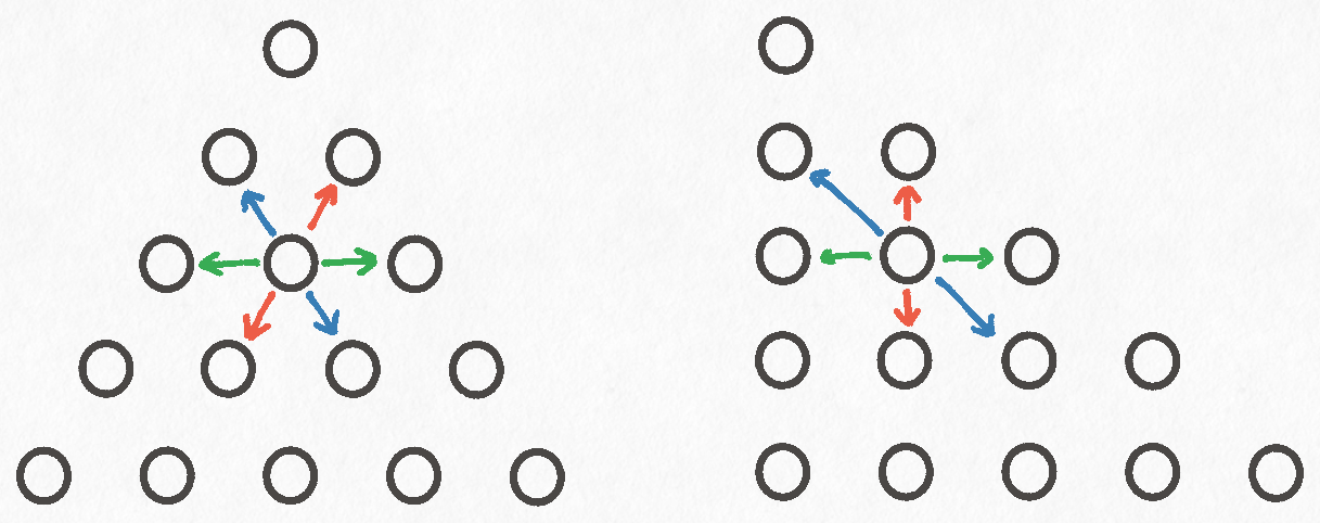
To make the board easier to reason about, let's realign it so that it's drawn as a right triangle instead of an equilateral one. This redrawing doesn't change anything about the game, but it makes it easier to see which cells are related to each other by neatly arranging things on a grid.

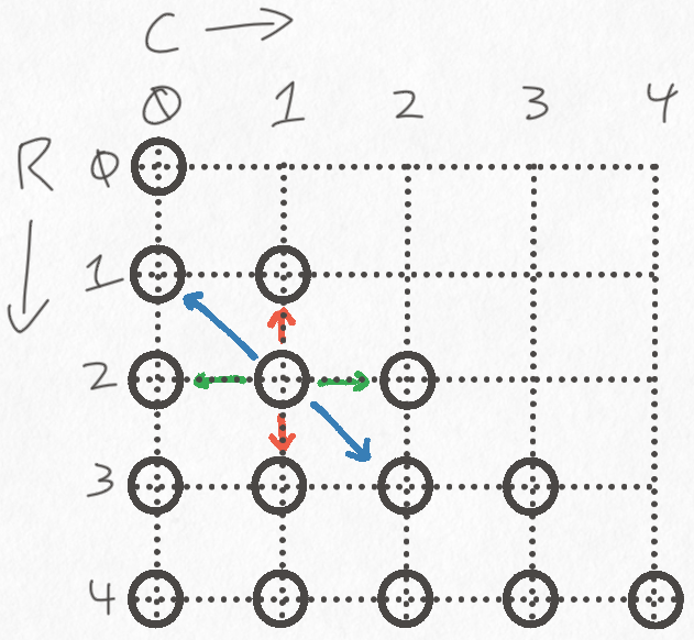
In order to describe to a computer how to play the game, we'll have to come up with some concrete notation for describing the moves. A great first step is to notate every cell with a coordinate. We'll number the rows of the board from top to bottom, starting with row 0. In each row, we'll number the cells in that row from left to right, also starting with 0. These two numbers uniquely identify the row and column of every cell on the board.

Distorting the board into a right triangle reveals that pegs can move in three directions:

1. Up and Down
2. Left and Right
3. Along the hypotenuse of the triangle

Moving up and down corresponds to incrementing or decrementing the value of the "row" axis. Similarly, moving left and right is incrementing or decrementing the value of the "column" axis. Finally, moving along the hypotenuse of the triangle involves incrementing or decrementing both the "row" and "column" axes simultaneously.

This coordinate system is enough for us to describe every possible move on the board, so we can move on to figuring out how to represent the board in memory.

In-Memory Representation

Jagged Arrays

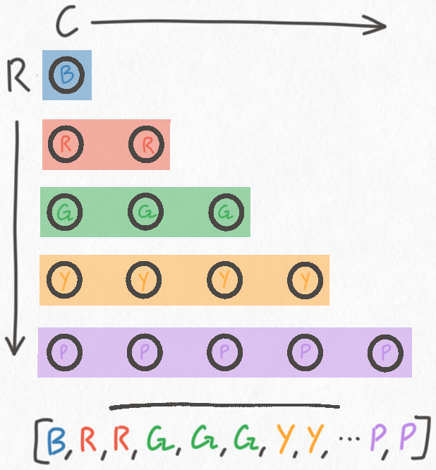
One way we could store this structure in memory is with a jagged array. The first sub-array would represent the first row and consist of only one element. The second sub-array would represent the second row and consist of two elements, etc. In Rust we'd do this with Vec<Vec<u8>> (list of lists of bytes). This is a very natural choice because it visually matches how we draw the board very closely.

The problem with any array based approach is that you end up wasting a lot of memory. For each cell on the game board, we only need 1 bit of data: whether the cell is occupied by a peg or not. However, all memory allocated on a computer will be allocated using some number of bytes. You can't allocate a fraction of a byte, as a simple fact of how CPUs are designed.

As a consequence, the smallest a single Vec element can be is a byte. So, if we were to use something like this to store our game board:

// Note how closely this parallels the drawings from earlier.
let board: Vec<Vec<u8>> = vec![
    vec![0],
    vec![1, 1],
    vec![1, 1, 1],
    vec![1, 1, 1, 1],
    vec![1, 1, 1, 1, 1],
];

We would be using at least 15 bytes plus the memory used by each Vec to track its own capacity and length. Fortunately, Rust provides a size_of function that we can use to find that out. Calling size_of::<Vec<u8>>() returns 24, meaning that an empty Vec<u8> consumes 24 bytes. This number is going to vary by platform, but it's probably going to be the same for all 64-bit system architectures.

So, if each Vec consumes 24 bytes just by existing, a jagged Vec board will consume 159 bytes of memory. 15 bytes for the cells of the game board, and then 144 bytes for all of the Vec instances.

This is not very efficient! Over 90% of the memory is taken up by the internal state of each Vec. If you also consider the waste of allocating a full u8 for each board slot, a ragged Vec is only about 1% efficient.

Flat Representation

A good starting optimization is to flatten out the board into a single Vec. That is, instead of having a Vec per row, and an outer Vec to group it all together, we instead store the entire board in a single Vec.

This certainly saves a lot of memory. A flat Vec only consumes 39 bytes. However, it's not immediately obvious how we'd interact with this structure. With a ragged Vec, it's clear how to use our row/column coordinate system. The cell at coordinate $(r,c)$ is given by: board[r][c].

Fortunately, it's pretty easy to convert from (row, column) coordinates to an array index and vice-versa.

Let's begin by defining a Coordinate struct and implementing a constructor that prevents us from creating invalid coordinates:

#[derive(Eq, PartialEq, Debug, Copy, Clone)]
pub struct Coordinate {
    r: usize,
    c: usize,
}

impl Coordinate {
    pub fn new(row: usize, col: usize) -> Option<Coordinate> {
        if col <= row {
            Some(Coordinate { r: row, c: col })
        } else {
            None
        }
    }
}

For those who don't know Rust, usize refers to an unsigned integer that is large enough to refer to any location in memory. So, on a 64-bit system it's 64-bits. Because a usize is always large enough to refer to any memory address, it's the type used when indexing into things like arrays.

Next, we want to be able to convert between array indices and Coordinate instances. We'll start by defining a function called row_offset which accepts a row index and returns the index that corresponds to the start of that row in a flattened representation of the board.

fn row_offset(r: usize) -> usize {
    // The lower-bound needs to be 0 in-case
    // `r` is 0.
    (0..=r).sum()
}

Lets step through an example of how this works. Suppose we want the start index of the row with index 3:

0 <-- row 0
0 0
0 0 0
0 0 0 0 <-- row 3, starts at index 6
0 0 0 0 0

Because the rows are 0-indexed, we know that there will be 3 rows before the start of our target row. Counting how many elements exist before the start of our target row is thus a matter of summing the numbers 0 through r. As noted in the code sample, we start summing from 0 so that the function has a well defined value in case we compute the row_offset of row 0.

Once we have the start index of the row, we can add the column coordinate to get the final index. For example, the cell (3, 2) is row_offset(3) + 2 or index 8. This is implemented in the following method:

impl Coordinate {
    pub fn to_idx(self) -> usize {
        row_offset(self.r) + self.c
    }
}

With Coordinate to usize conversion out of the way, we can implement conversion in the other direction. Given an index, finding the column is easy since we already have row_offset. Since the row_offset is the number of elements present before the start of an element's row, the column of an element at index i is given by i - row_offset(i).

Finding the row requires some new code that basically amounts to counting:

pub fn row_of_idx(idx: usize) -> usize {
    // Rather inelegant but should be pretty fast

    let mut j: usize = 0;
    let mut r: usize = 0;
    let mut cells_per_row: usize = 1;
    let mut cells_left_in_row: usize = 1;

    // We count along until we reach the target index
    while j < idx {
        // Every time we move a space, we're consuming a cell in this row
        j += 1;
        cells_left_in_row -= 1;

        // If we're out of cells, then we've gone through an entire row.
        if cells_left_in_row == 0 {
            cells_per_row += 1;
            cells_left_in_row = cells_per_row;
            r += 1;
        }
    }
    r
}

With this function in hand, we can implement our conversion function:

fn from_idx(idx: usize) -> Coordinate {
    let r = row_of_idx(idx);
    let prior_elements = row_offset(r);
    let c = idx - prior_elements;

    Coordinate { r, c }
}

To be extra fancy, we use these functions to implement From, which will let us write functions that can accept either a usize or a Coordinate and convert between them as necessary.

// Replaces the `Coordinate#to_idx` method
impl From<Coordinate> for usize {
    fn from(c: Coordinate) -> usize {
        row_offset(c.r) + c.c
    }
}

// New code:
impl From<usize> for Coordinate {
    fn from(idx: usize) -> Coordinate {
        let r = row_of_idx(idx);
        let prior_elements = row_offset(r);
        let c = idx - prior_elements;

        Coordinate { r, c }
    }
}

Now that we can convert between (row, column) coordinates and flat indices, we can store the board as a flat Vec and use whichever coordinate system is most convenient in any given situation.

A flat Vec bumps us from 1% efficiency to roughly 5%, which is an improvement, but a relatively meager one. Fortunately, it turns out we can do even better.

Even More Efficient!

The key issue is that each cell in a Vec based board is going to waste the vast majority of its memory, on account of each cell being a full byte when only one bit is required.

Instead of using a Vec, what if we stored the board as an integer, where each bit of the binary representation represents a cell? We can totally do that and save even more memory! Instead of using methods from Vec to look at each cell in the board, we'll use bitwise operations to inspect and set individual bits of the number, and in the end accomplish the same thing.

An unsigned 64 bit integer will let us store boards with up to 10 rows (55 cells) using only 8 bytes. In comparison, a 55 cell Vec would consume 79 bytes on my computer, so this is substantially more efficient!

For practicality's sake we should also store the number of rows in the board, as well as the number of cells, so our final struct will look like this:

struct Board {
    rows: u8,
    cells: u8,
    state: u64,
}

We don't need to worry about overflowing rows or cells because the maximum number of cells we can represent in a u64 is (no big surprise) 64, which will definitely not exceed rows or cells.

At first blush, one might assume that Board is 10 bytes large. However, because of how Rust lays out structs in memory a Board actually consumes 16 bytes. 8 of those bytes store the state field, rows and cells consume 1 byte each, and the rest is padding.

This means that our integer based board is 12.5% efficient, since the entire struct is 16 bytes and we only need 2 of them to store the default 5-row board.

If we really wanted to optimize, we could swap the u64 for a u16, which cuts the size of the struct down to 4 bytes. At that point the representation is about as efficient as possible without forgoing a struct altogether and using a raw u16. However, if we were to use a u16, we'd only be able to explore the 5-row version of the game, which is small enough (in terms of possible moves) that memory efficiency just doesn't matter that much. Storing the board in a u64 does waste some memory, but it means I can write the code once and be able to explore all sizes of the game up to 10 rows. That's fine enough, because the game starts to become computationally infeasible around 10 rows anyway.

It's theoretically possible to tell Rust to lay out the struct without padding, but the documentation strongly recommends against tuning struct layout unless you have a good reason to do so. Removing the padding is quite likely to make the program slower by messing up memory alignment, so I'm going to quit while I'm ahead and not mess with things I don't understand.

Treating a u64 like a Vec

Earlier I mentioned that we could use bitwise operators to act on the integer like it's an array of bits. Let's look at how:

impl Board {
    fn set_coordinate<C: Into<Coordinate> + Into<usize>>(&mut self, c: C) {
        let cell_digit: usize = c.into();
        // 000...1...000
        let mask: u64 = 1 << cell_digit;
        self.state |= mask;
    }

    fn clear_coordinate<C: Into<Coordinate> + Into<usize>>(&mut self, c: C) {
        let cell_digit: usize = c.into();
        // 111...0...111
        let mask: u64 = !(1 << cell_digit);
        self.state &= mask;
    }

    fn check_occupied<C: Into<Coordinate> + Into<usize>>(&self, c: C) -> bool {
        let cell_digit: usize = c.into();
        let mask: u64 = 1 << cell_digit;
        (self.state & mask) != 0
    }

    fn check_empty<C: Into<Coordinate> + Into<usize>>(&self, c: C) -> bool {
        !self.check_occupied(c)
    }
}

Immediately there is some hairiness with the generic type for C. Earlier, the conversions between row/column coordinates and flat indices were defined using the From trait. Rust automatically provides implementations of Into if you implement From, and so what this boils down to is that these methods can be called with either a Coordinate or a usize. The into method will call the proper conversion method based on the type annotations, or if no conversion is necessary (the value is already of the desired type) no conversion will be performed at all.

The next difficulty, if you're unfamiliar with bitwise operations, is the left shift operator, denoted by <<. The left shift operator, as the name implies, shifts all of the binary digits of a number a certain number of places ot the left. Any digits that go off the left side of the number are discarded, and new zeros are added on the right hand side, as necessary. For example:

let ex: u8 = 0b01100001;
let shifted: u8 = ex << 3;
// Shifted is:
// 0b00001000
// The 1s at the end of `ex` "roll off"

The line of code: let mask: u64 = 1 << i is creating a number where every digit of the binary representation is a 0 except for the digit at index $i$. The ! operator flips every binary digit, so !(1 << i) is similar except the digit at index $i$ is a 0 and every other digit is a 1.

The final ingredient here are bitwise-and and bitwise-or. Let's take set_coordinate as an example. Suppose we want to set the cell at index 3, note that index 0 corresponds to the least significant digit and is therefore all the way to the right. Also, for the sake of brevity, I'll be writing out the examples as 1 byte even though the real board consists of 8 bytes.

board = 1011 0011
mask  = 0000 0100
(perform logical-or between each pair of digits)
board = 1011 0111

The reason that this works is because x OR 0 == x and x OR 1 == 1 regardless of whether x is 1 or 0. The exact same logic is used for clearing a specific index. Except instead we rely on the fact that x AND 1 == x and x AND 0 == 0, and we use an inverted mask.

Finally, to check if a specific index is occupied, we use a mask as if we're setting a cell, but perform a logical-and instead. This clobbers out every digit except for the one we want to introspect. If that digit was a 1, then it will be preserved in the logical-and. If the digit was a 0, then it will be destroyed along with every other digit, which we can easily detect.

board = 1011 0011
mask  = 0001 0000
logical-and
res   = 0001 0000
-----------------
res != 0 so the bit
at index 4 is occupied

Graph Representation

Now that we have a way to represent the board in memory, we can define how we'll store the entire game graph. The simplest data structure we can get started with is the adjacency list, which I implemented as: Vec<(Board, Vec<Board>)>. Each entry in the outer Vec represents a node in the graph. The first element of the tuple is the data contained by the node, and the second element of the tuple is a list of the node's neighbors. Conveniently, the Board type has simple by-value equality (two Board structs are equal if their individual fields are equal), so we don't need any extra machinery to tell the difference between boards or otherwise perform node lookups.

Generating the Graph

For the sake of brevity, and because I'll be open-sourcing the Rust implementation, I'm going to describe the algorithm involved in pseudocode. There are some interesting details involved in keeping the implementation ergonomic, but the actual work the code is doing is conceptually boring, so I wont spend time covering it.

The following code generates the game graph from the given start board in a depth-first fashion. The pseudocode is almost the same as the actual Rust implementation, but I've taken the liberty of removing implementation details and coming up with some imaginary functions to make the algorithm itself read more clearly.

type GameGraph = Vec<(Board, Vec<Board>)>;

pub fn build_graph_from(start: Board) -> GameGraph {
    let mut graph: GameGraph = Vec::new();
    let mut processed: HashSet<u64> = HashSet::new();

    // A stack containing nodes we need to process.
    // The core difference between DFS and BFS is swapping 
    // this stack for a queue.
    let mut frontier: Vec<Board> = vec![start];

    // For non-Rust programmers, this loop will continue
    // to pop boards off the frontier until the frontier
    // is empty.
    while let Some(board) = frontier.pop() {
        // It's possible for us to see nodes we've already processed
        // but because of the properties of DFS we know that any node
        // in the processed set has already been fully explored. That
        // is, this node, its neighbors, its neighbor's neighbors, etc.
        // have already been processed. So, we can skip it.
        if processed.contains(&board.state) {
            continue;
        }

        let mut neighbors: Vec<Board> = Vec::new();
        // `move` is a reserved word in Rust, so we can't use the 
        // obvious name.
        // check every possible move on this board, and if a move
        // is valid, generate what the board would look like if
        // we made that move and add it as an edge.
        for m in all_moves_from(board) {
            if is_valid(m, &board) {
                let n = board.apply_move(m);
                neighbors.push(n);
            }
        }

        processed.insert(board.state);
        graph.push((board, neighbors.clone()));

        // Continue exploring this section of the graph
        for n in neighbors {
            frontier.push(n);
        }
    }

    return graph;
}

The graph generation is a standard depth-first traversal where the neighbors are generated on the fly.

The main thing I want to explain about this algorithm is why we check for nodes we've seen before and why we can be confident in skipping them.

Imagine we have a graph with three nodes in it. One node represents the start of the game and it has two neighbors representing two possible moves you could make. Let's call these two moves L and R and the start move S. I'll also use notation like Lx or Rx, where x is a counting number, defined as: "Lx and Rx mean a board found x moves away from L or R respectively".

When we start the algorithm, the frontier contains one node: [S]. Once we explore S we will discover its two neighbors and the frontier will contain two nodes: [L, R].

Because the frontier is operating as a stack, we will explore R first and the frontier will be updated with the neighbors of R: [L, R, R1, ... R1]. Then we will explore the first neighbor of R and put its neighbors on the stack: [L, R, R1, ..., R1, R2, ..., R2]. This process will repeat until every board reachable from R has been explored, and only then will L be explored. In this sense exploring is "total": If a node has been visited then we know that every subsequent board reachable from that node has also been processed.

It's conceivable that two different sequences of moves could eventually converge back into the same board state. So, over the course of exploring L we may end up generating a neighbor that we have already seen. Because we know that previously visited nodes have been completely explored, there is no reason to process that node again. However, we do need to be careful that we don't accidentally discard edges in our graph. If we re-encounter a node, we want to record the new edge that points to that node, but not continue the traversal from that node.

What's Next

I've omitted some details of the implementation because they're entirely concerned with the fiddly, but otherwise simple and uninteresting, process of generating every possible move on a given board. As mentioned previously, I'll be open sourcing all the relevant code once this series of posts is complete, if you're curious about what I've left out.

Next time, we'll being using this implementation to answer questions about the game. In particular, I want to examine how difficult the game actually is and whether it seems to get easier or harder as you increase the size of the board.