Southern Food and Graph Theory: Part 4

Once again, the calendar snuck up on me and I realized that 2025 is almost over and I've not finished this series of posts. I really thought they would've been done by now, but frankly I procrastinated too much and now here I am, rewriting this post from scratch in the middle of December.

I'm going to start with a few interesting diversions I took while working on this project, and then we'll get into the actual analysis of the game!

Memory Optimizations

The size of Peg Solitaire grows quite dramatically as you add rows to the board, so I quickly found it necessary to do some more code optimization in order to explore larger boards.

For some perspective, the default 5-row version of the game produces a graph with around 3,600 nodes. Now, simply add two rows to the board, and you're looking at ~40 million nodes. Add one more row, and the number of nodes jumps to many hundreds of millions.

At these scales, memory usage quickly becomes a problem, and so the representation of the game board and the graph as a whole needed revisiting.

Recall that the Board struct we left off with was set up like so:

struct Board {
	state: u64,
	rows: u8,
	cells: u8
}

Due to memory alignment requirements, Rust pads out this struct to 16 bytes. This means that every Board the program allocates has 6 bytes of literally empty space! No good!

Because the state property has 64 bits, the largest board we can store has 10 rows. Once you get to 11 rows, the board has 66 cells and would require a larger integer to store. Strictly speaking, Rust does have a u128 type, but I don't think it's computationally tractable to go much larger than 10 rows, at least for the things I'm doing, so there's not much point.

Now, a 10 row board has 55 cells. This means that the top 9 bits of Board.state are never used for anything. So, what if we stored the number of rows in those top 9 bits? That's great and all, but if we don't get rid of rows and cells we're still going to end up allocating 16 bytes.

Fortunately, because we're capping the number of rows at 10, we can just precompute the number of cells in a board with N rows and store it in a static array. At runtime, if we need the number of cells in a board, we can perform a lookup into that array to get the correct number of cells.

By packing rows and state into the same u64, and looking up cells at runtime, we reduce the board struct to a wrapper around a single u64 and cut the size in half! Great success! Here's what it looks like in practice:

#[derive(Debug, Copy, Clone, Eq, PartialEq, Hash)]
pub struct Board(u64);

const ROW_OFFSET: usize = 56;

/// AND this with the packed state to get the cell count.
const ROW_COUNT_MASK: u64 = 0b11111111 << ROW_OFFSET;
  
/// AND this with the packed state to get the cell values.
const BOARD_MASK: u64 = u64::MAX >> 9;

// This is the `cells` lookup array. It's a bit oversized but
// it makes me feel better to have it that way.
static TRIANGULAR_NUMS: &[u8] = &[0, 1, 3, 6, 10, 15, 21, 28, 36, 45, 55, 66];
  
impl Board {
    pub fn new(rows: u64) -> Board {
        if rows > 10 {
            panic!("10 rows is the maximum board size that can be represented with a u64!");
        }
        // Stash the number of rows in the top 8
        // bits but leave everything else 0 to start.
        Board(rows << ROW_OFFSET)
    }
  
    // For debugging
    pub fn packed_state(&self) -> u64 {
        self.0
    }
  
    pub fn state(&self) -> u64 {
        // 0000000001...1
        self.0 & BOARD_MASK
    }
  
    pub fn rows(&self) -> u8 {
        // First, we mask out the row count
        // Then we shift the bits back down
        // to little end and cast to u8.
        ((self.0 & ROW_COUNT_MASK) >> ROW_OFFSET) as u8
    }
  
    pub fn cells(&self) -> u8 {
        TRIANGULAR_NUMS[self.rows() as usize]
    }
  
    /// Returns the number of pegs on the board.
    pub fn order(&self) -> u32 {
        self.state().count_ones()
    }
  
    /// Overwrites the entire board.
    pub fn set(&mut self, new_state: u64) {
        let num_cells = u64::from(self.rows());
        self.0 = new_state | (num_cells << ROW_OFFSET);
    }
    
    // All of the other operations on the Board are essentially
    // the same, so I'm omitting them for brevity.
}

The BOARD_MASK and ROW_COUNT_MASK are inverses of each other (honestly they should probably be defined that way). In the case of the BOARD_MASK, the top 9 bits are zeros and everything else is a 1, so if you bitwise-and that mask with the Board, any ones in the top 9 bits are canceled out, and any set bits in the bottom 55 bits are preserved. The ROW_COUNT_MASK is the exact same idea, just inverted so that the top 9 bits are the ones that get saved. After you mask out the row count, you have to shift the bits down to the right, so that you read out the correct decimal value:

// I actually only use the top 8 bits so that row_count
// is still a byte, like it was in the original struct.
00001010 ...the rest of the number...
111111111000....0000 < the mask
BITWISE_AND---------
000010100000....0000
// Then right shift...
000...0001010 = 10 in decimal

We have to define methods for getting the state, rows, and cells values, and we have to be mindful when overwriting the entire board state. Otherwise, very few code changes are required and we get the benefit of using half as much memory! At this point, I called it quits optimizing Board, because I have no clue how it could get any smaller (Doesn't mean it couldn't get smaller! Just that I don't know how to do it).

With Board handled, there is another glaring inefficiency in the GameGraph type that needs to be handled. Recall that GameGraph is defined as:

type GameGraph = Vec<(Board, Vec<Board>)>

Each element in the GameGraph represents a node and a list of nodes that are adjacent to it. On my system, Vec uses 24 bytes just to exist. In a graph with many millions of nodes, this adds up very quickly. Can this be made more efficient?

Well, the reason that Vec takes up that space in the first place is that it's resizable, and it needs that memory to perform various bookkeeping. However, in our situation, the list of edges is immutable! Once we create it, we never touch it again, so all that machinery to support runtime resizing is wasted in this situation.

Instead of storing the edges in a Vec, we can store them in a plain old fixed-size array. This removes the memory overhead introduced by the Vec.

At this point I could go on a long tangent about sized VS unsized types in Rust, Box, slices, etc. But frankly, this post is already quite long, and so I'm going to show the outcome of the optimization, and leave it as an exercise for the reader to decipher why the types are the way they are. The upshot for this post is that Box is an 8 byte pointer instead of a 24 byte Vec, and it lets us use the fixed-size array without the Rust compiler having a (very justified, mind you) cow.

The change ends up being rather simple. First, the type signature for GameGraph needs to change:

type GameGraph = Vec<(Board, Box<[Board]>)>

Then, there are a few mechanical and boring type signature changes from Vec<Board> to Box<[Board]> that are omitted for brevity.

Finally, we need to update the line of code that adds nodes to the GameGraph:

// Change this:
graph.push((board, neighbors.clone()));
// Into this:
graph.push((board, neighbors.clone().into_boxed_slice()));

The into_boxed_slice method converts a Vec<T> into a Box<[T]>, which is exactly what we want! We still have to clone because we want the graph to be able to own the list of edges, but the boards are just wrappers around u64, so this cloning is very cheap.

Let's tally up all the optimizations! Previously, a single node in the graph, a (Board, Vec<Board>), consumed 40 bytes plus 16 bytes per edge. Now, a (Board, Box<[Board]>) consumes 16 bytes plus 8 bytes per edge, a substantial improvement!

Performance Optimization

Something else that needed to be tuned was the data structure used by the GameGraph itself. To this point, I've stored the graph as a Vec, which has worked fine and has the neat property of preserving the graph's topological ordering. However, a majority of graph algorithms require you to be able to look up a node's neighbors. The way GameGraph is defined today, this lookup will take $O(n)$ time with respect to the number of nodes. So, instead of using a Vec, we can use a HashMap. This lets us perform neighbor lookups in constant time, which is what we want. We can also emulate having the Vec by iterating over the map's entries (key-value pairs), so all we lose is the explicit ordering of the Vec, which we didn't really need anyway.

Changes throughout the codebase are very small and mechanical, so I wont detail them here.

Graph Visualization

Another diversion I got up to in this project is visualizing the graphs. They didn't turn out nearly as nice as I wanted, but they still have some explanatory power and are pretty to look at regardless.

Let's start with the 4-row version of the game, because its graph is small enough that you can actually tell what you're looking at.

A figure showing the game graph for the 4-row version of the game. — The 4-row game graph

This graph, while relatively puny, illustrates several features that are common to all of the peg game graphs, namely:

The layered structure that is a result of the graph being a DAG.
The rough "diamond shape" where the the middle layers of the graph generally have more nodes.
The interwoven nature of the layers, where there are often many ways to reach a particular board state, even when looking only at adjacent layers.

The number inside each node is the numeric representation of the board's state. With this fact in mind, the eagle-eyed among you will have concluded that this particular graph has no winning states, since a state with 1 peg would naturally have to be a power of 2 when converted to decimal.

For anything larger, I failed to figure out how to visualize the graphs the way I wanted. GraphViz could handle at least the 5-row graph, but produced an image that was both extremely large and also unintelligible. Another tool I found, Gephi, handled the larger graphs somewhat well but lacked the functionality to do a layered visualization. Gephi does have a GraphViz plugin that I tried, but I couldn't get it to work.

So instead, enjoy an interesting looking but otherwise completely meaningless picture of the 5-row game graph, if only to get a sense of its scale:

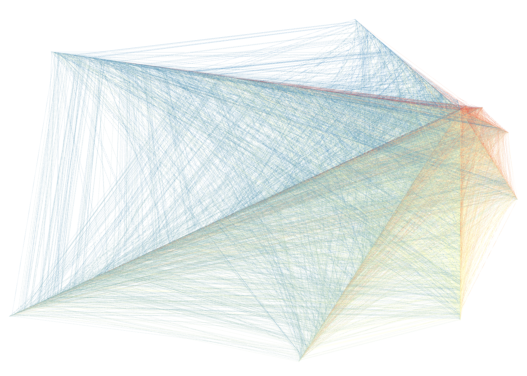
A fuzzy picture of the five row game graph. The nodes are color coded and sorted by how many edges start at that node. This results in a star-like shape. — 5-row game graph

The nodes are color coded and sorted by their "out-degree", which is how many edges start at that node. I don't think there's much to learn from this graph, it's just pretty.

Back to the Point

Memory optimization and visualization are fun and all, but they weren't the point of this intensely drawn out project. My mission was to figure out if Cracker Barrel was justified in calling me a dummy for leaving 2 or 3 pegs on the board while waiting for my chicken fried steak.

To do this, we have to decide what we mean by "difficulty". We've got to come up with some sort of computable metric. Ultimately, difficulty is subjective and what makes a game difficult is not necessarily encoded in any particular model of its moves. As an exercise for the reader, try and come up with some games that could have arbitrarily complicated game graphs (constructed in the way I'm doing here for peg solitaire), while still being essentially trivial for a human to win. Or conversely, come up with a game that has a simple graph while still being tricky to solve.

What we can do is establish a relative difficulty between different variants of peg solitaire by repeatedly computing the metric in different situations. We can see if, all other things being equal, a particular starting position is easier than the others, or how much easier it is to end the game with 2, 3, or 4 pegs, compared to winning.

Some Possible Metrics

Let's look at some options, in order to help explain why I'm computing difficulty the way I am.

Node Counting

The simplest metric I can think of is to gather up all the "terminal nodes" in the graph, meaning all the nodes from which you can't make any more moves, and group them by how many pegs are left on the board. Once you have these groups, you can use the number of nodes in each group to come up with a notion of relative difficulty. For example, if you have 10 terminal nodes with 2 pegs but only 1 terminal node with 1 peg, then you might say that it's 10 times "as easy" to end the game with 1 peg.

While the simplicity of this metric is alluring, we can easily produce a counter example that shows it has some undesirable properties:

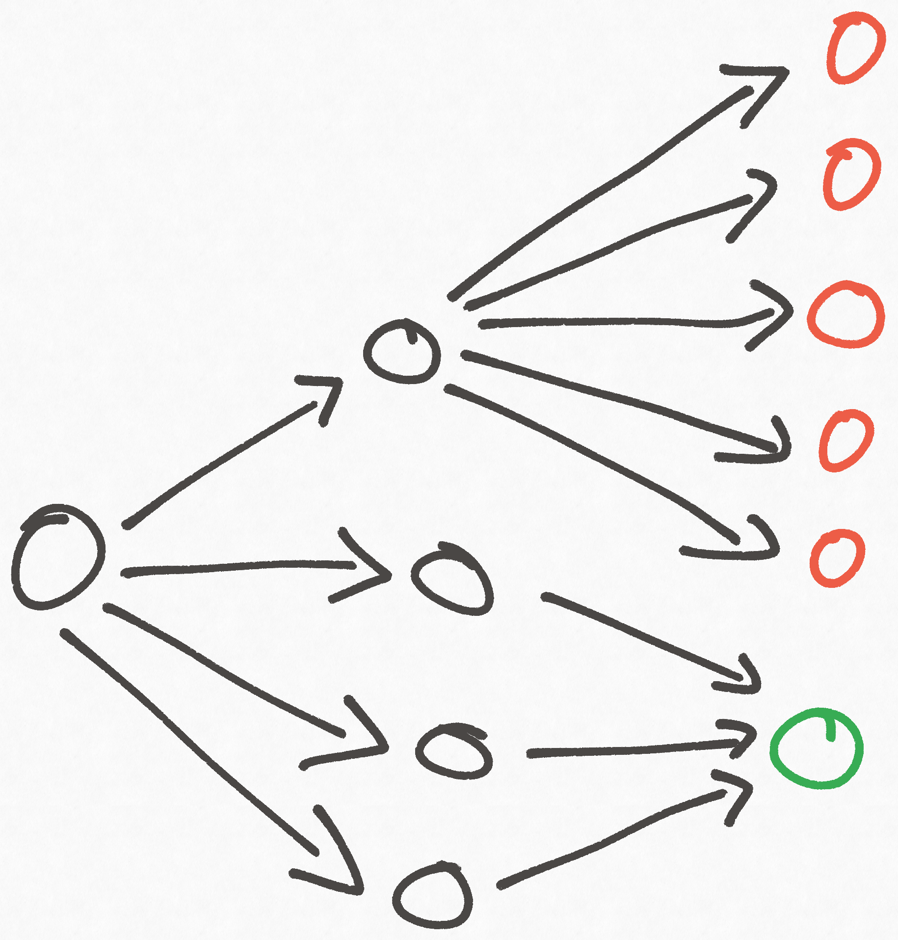
An example graph showing why node counting can produce incorrect results. — Node counting counter-example

Based on node counting alone, we'd conclude that the game is pretty hard because there are 5 times more losing nodes than winning ones. But when we take account of the whole graph, this conclusion doesn't make sense, because whether you win or lose only depends on the first choice you make, and there are three times more good choices as bad ones!

While we can't know ahead of time if this kind of structure exists in the graph we want to analyze, but supposing it did, this metric would give us a bogus result. Simply counting the number of terminal nodes with a particular property is not sufficient, because it makes no account of the connectivity within the graph that lets you reach those nodes.

Path Counting

In order to account for connectivity through the graph, we could instead count the number of distinct paths from the start node to terminal nodes of particular properties. For example, we could compare the number of distinct paths to terminal nodes with 2 pegs compared to terminal nodes with 1 peg.

This metric is unfortunately susceptible to a similar problem as node counting, which we can demonstrate with the following diagram:

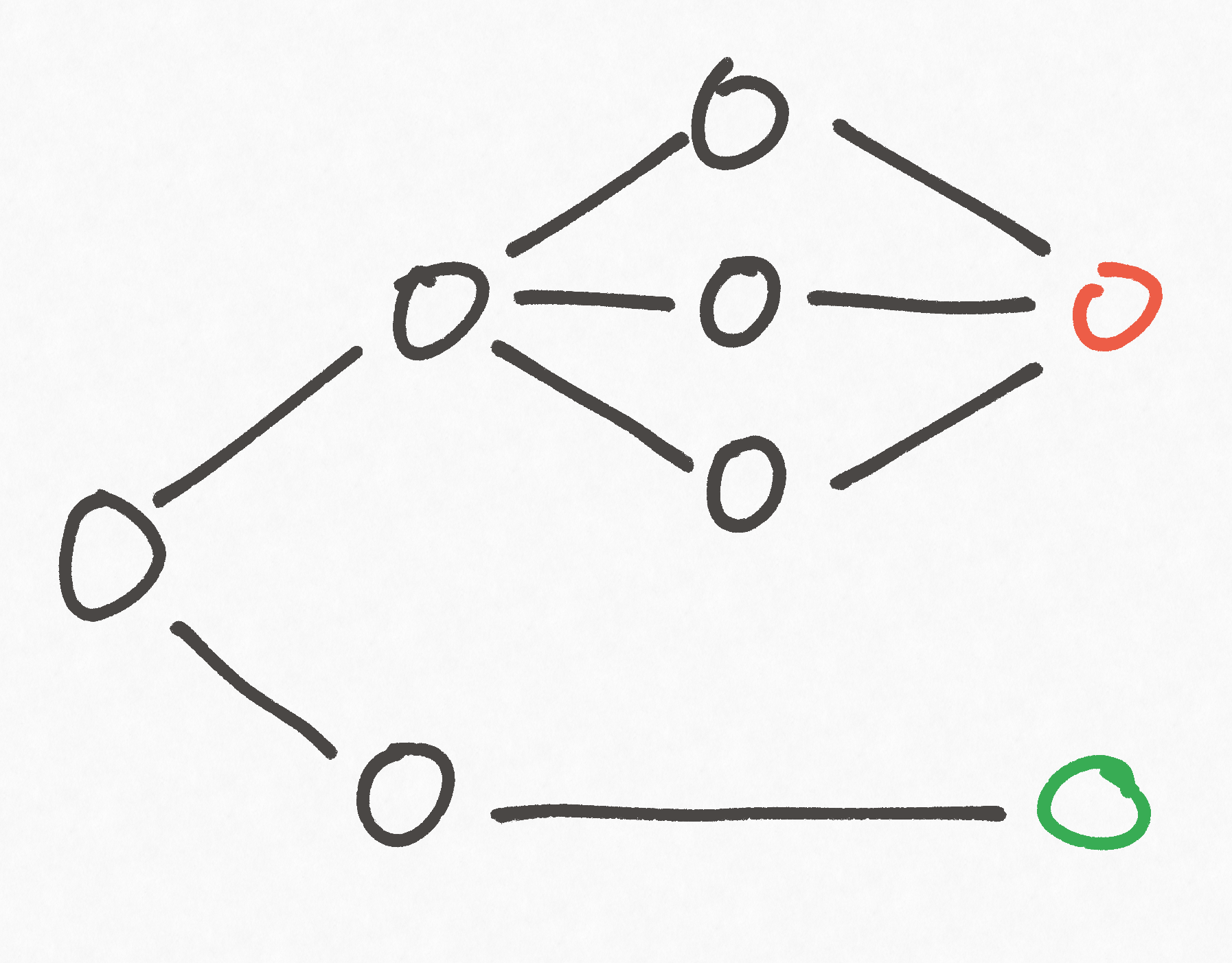
An example graph showing why path counting can produce incorrect results. — Path counting counter-example

In the example above, there are three paths to a losing node, but only one path to a winning node. Like in the node counting example, whether you you win or lose only depends on the first choice you make, and it's 50/50. So if we employed path counting to examine this graph we'd get a skewed result.

Additionally, this metric would also be pretty expensive to compute.

A Better Metric

We can't know for sure if these structures I'm producing as "counter examples" actually exist in the game graph. But the point is that even if these structures exist only partially, we're going to get skewed results from these strategies. Besides, it would be better if we could come up with a metric that's sound even in the face of arbitrary directed acyclic graphs, so that we can be more confident of the results.

Imagine the graph as a series of rooms connected by pipes. Lets think of terminal nodes as having taps/faucets in them. For the sake of the analogy, lets say that winning nodes emit water and losing nodes emit oil. These liquids flow through the pipes connecting adjacent rooms, and when they reach a room they produce a mixture of oil and water. This mixture then continues flowing through pipes, and mixes with the output of other nodes to produce a new mixture, and so on and so forth until the mixture reaches all the way back to the start node. At which point we can measure the proportion of oil and water to get an idea of how easy or difficult the game is

While this oil and water analogy captures the idea of this metric, it's not actually how we're going to define it in practice. In my opinion, the simplest implementation is a recursive one, with pseudocode something like this:

procedure difficulty_from(node, graph):
  if is_winner(node):
    return 1.0
  else if is_loser(node):
    return 0.0
  else:
    neighbors = graph.neighbors_of(node)
    num_neighbors = neighbors.len()
	total = neighbors.map(n -> difficulty_from(n, graph)).reduce(+)
	return total / num_neighbors

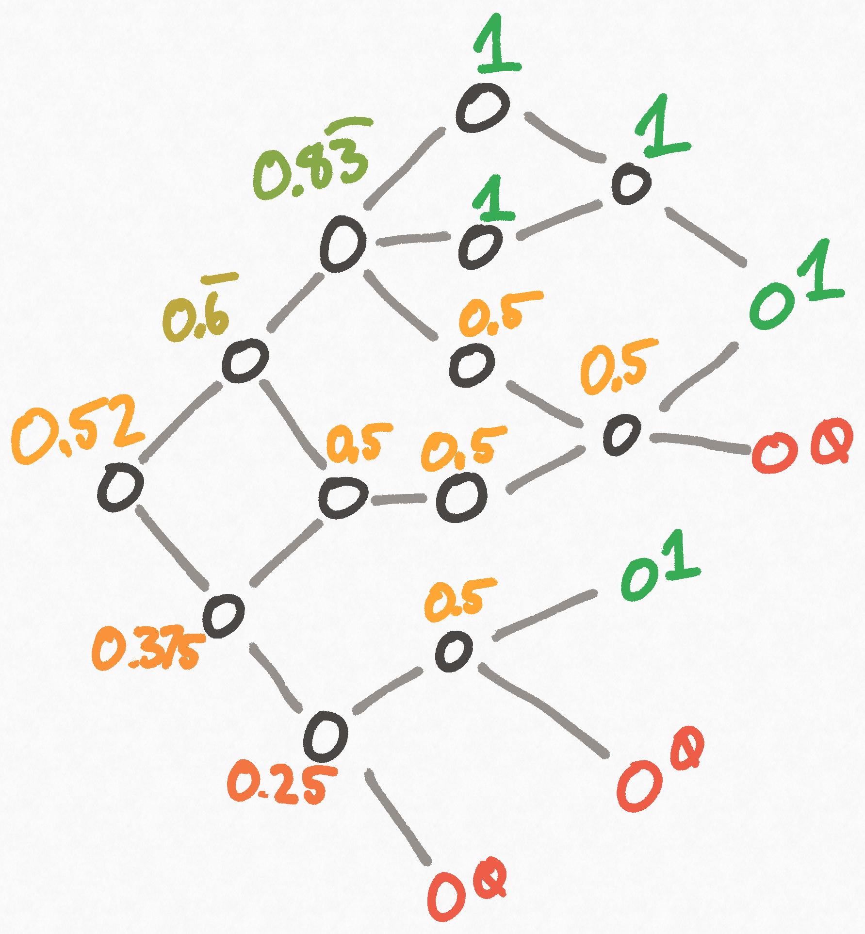
Put more plainly:

If you're a winning board state, your "difficulty" is a 1
If you're a losing board state, your "difficulty" is a 0
Otherwise, your difficulty is the average of all your neighbor's difficulties.

Strictly speaking, the term "difficulty" here is backwards, because intuitively difficulty should be lower when the number is lower. In reality, the game is harder the lower the number is. I could rename it, but I'm short on time getting this post out and renaming it sounds very tedious, so you'll have to bear with my laziness.

The implementation of this is pretty straightforward, though I suspect the recursion is relatively slow. We don't need to worry about the recursion depth getting too high because it's bounded by the number of cells in the board. Because each move in the game removes one peg, the length of the longest possible sequence of moves on a board is bounded by the number of pegs available. Since the largest board we can handle with this implementation has 55 cells, we wont make more than 55 nested recursive calls.

Here's a drawing to help visualize what this is doing:

A labeled example showing the recursive difficulty algorithm. — Recursive difficulty example

Now, if we translate this pseudocode directly into Rust and implement it, we'll find it is viciously slow. The reason for this is that we're actually duplicating a lot of work. As we proceed layer by layer through the graph, we only need to compute a node's difficulty rating once, at which point we can store it in a lookup table. If a node needs its difficulty computed again, then we can simply pull it from the table.

With that in mind, the full Rust implementation looks like this:

type DifficultyIndex = HashMap<u64, f64>;

fn compute_node_difficulty(b: &Board, g: &GameGraph, diff_idx: &mut DifficultyIndex) -> f64 {  
    // If this node has already been computed, just return the result.  
    if let Some(diff) = diff_idx.get(&b.state()) {  
        return *diff  
    }  
	
    if b.order() == 1 {  
        diff_idx.insert(b.state(), 1.0);  
		  
        1.0  
    } else if neighbors_of(b, g).is_some_and(|n| !n.is_empty()) {  
        let neighbors = neighbors_of(b, g).unwrap();  
        let total: f64 = neighbors.iter()
	        .map(|n| compute_node_difficulty(n, g, diff_idx))
	        .sum();  
			  
        let difficulty = total / neighbors.len() as f64;  
		 
        diff_idx.insert(b.state(), difficulty);  
        difficulty  
    } else {  
        diff_idx.insert(b.state(), 0.0);  
        0.0  
    }  
}

Then we wrap compute_node_difficulty with another function to make calling it more convenient:

pub fn propagate_difficulty(g: &GameGraph, start: Board) -> DifficultyIndex {  
    let mut index: DifficultyIndex = HashMap::new();  
  
    compute_node_difficulty(&start, g, &mut index);  
  
    index  
}

And just like that, we're in business!

The Data

After many thousands of words, we can finally start looking at some results! There are many different dimensions that could be looked at here, but honestly I'm tired of writing and thinking about this topic so I'm going to scope myself rather narrowly to the questions I introduced way back in part 1:

How much easier is it to end with 2, 3, or 4 pegs compared to winning the game?
What's the most number of pegs you can leave on the board without being able to make any more moves?
Which starting position is the easiest?
Are there unreachable board states?
As you increase the size of the game board, does the game get easier or harder?

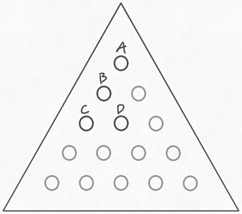
For clarity, I'm going to refer to the starting position where the corner of the board is empty as "standard position".

Let's start with a very basic analysis and look at the number of nodes and edges in the graph, starting from standard position, as we increase the size of the board:

Rows	Nodes	Edges
1	1	0
2	1	0
3	4	3
4	42	66
5	3,016	10,306
6	291,987	1,858,848
7	40,600,768	404,470,378

The game graph grows exponentially as we increase the number of rows, which explains why so many memory optimizations were necessary. Even after all the optimization, the 7-row game still consumes approximately 4 gigabytes of memory! Now, between 5 and 7 rows, the memory requirement goes up by a factor of 100-200x every time you add a row, so a conservative estimate on the size of the 8-row board is 388 gigabytes! Unsurprisingly, I don't have that much RAM, so we're gonna have to stop at 7 rows.

Using just these numbers, we can already answer a question: "Are there unreachable board states?" Emphatically yes.

Taking the 5-row game as an example, it has 3,016 nodes. But there are 32,766 possible valid boards, which means that not only are there unreachable boards, ~90% of all boards are unreachable! The effect is relatively consistent for 6 and 7-row games, where ~85% of boards are unreachable.

This exponential pattern allows us to make an educated guess about how difficulty scales. My guess is that it's dramatically easier (if not exponentially easier) to end with game with progressively more pegs, up to a certain point. This is because of the combinatorics of the situation. There are at most 15 unique boards that leave 1 peg in the 5-row game, but there are 105 ways to leave 2 pegs, and 455 ways to leave 3 pegs, etc. Because the number of combinations goes up so quickly, I'm guessing that it's much easier to stumble into one of these situations compared to winning the game.

The reason this effect only extends to "a certain point" is that once you have too many pegs on the board, you still have moves you can make and so the game isn't finished.

Furthermore, based on the exponential increase in the size of the graph as you add rows, I'm going to guess that the game gets harder as you add rows. But enough speculation! Let's look at some data!

For brevity I've labeled the 4 starting positions as A, B, C, and D:

An image showing which start positions correspond to which labels. The corner is A, the slot down and to the left is B, down and to the left again is C, and to the right of C is D. — Labeled starting positions

Here's a somewhat wonky chart where each row corresponds to a starting position, and each column corresponds to a particular number of pegs on the board we're targeting.

5-Row	1	2	3	4
Start
A	0.0069	0.0651	0.3196	0.7908
B	0.0034	0.0416	0.2866	0.7499
C	0.0071	0.0747	0.3450	0.8008
D	0.0017	0.0373	0.1878	0.7249
AVG	0.0048	0.0547	0.2847	0.7666

The game gets much easier as we target more and more pegs, which lines up with our prediction. And to answer another one of our questions, starting with the empty slot in the middle of one of the edges (position C) gives you a moderate advantage over the other options.

Now, I didn't collect numbers for anything past 4 pegs, because almost every time I've played (or seen this game played), you end up with no more than 4 pegs. But, in theory, what's the worst you could do at the game? In my opinion, it's not obvious from just thinking about it, and it's very easy to check by computer.

It turns out, that in the 5-row game, the worst you can do from standard position is 8 pegs left. From the B starting position, you can do slightly worse and leave 10 pegs. Interestingly, this number doesn't get much higher as you increase the size of the board. I didn't check thoroughly, but the highest numbers I saw for the 6 and 7-row games were 12 and 18 pegs respectively.

This leaves us with but one question remaining. Does the game get easier or harder as you make the board larger? This is where we encounter a surprising result! The 6-row game actually is easier than the 5-row game, unless you're trying to end the game with 4 pegs.

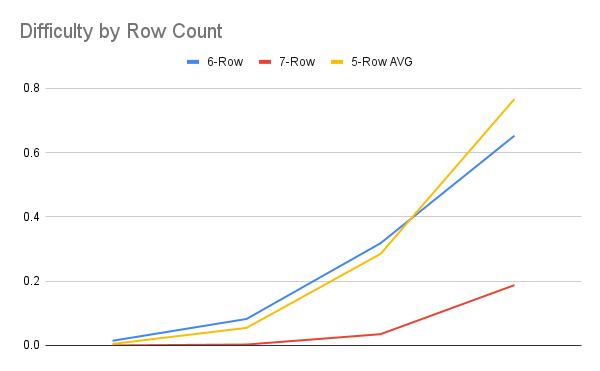
A chart showing the difficulty metric scaling for different board sizes. — Chart showing the difficulty scaling for various board sizes as you end the game with different numbers of pegs.

This is a very unintuitive result, considering that the 7-row game is substantially more difficult than either the 5-row or 4-row. In fact, the 7-row game doesn't even have solutions from standard position! You have to start from position B to have any chance of winning. Barring a bug in my code, I don't have a great explanation for why the 6-row game appears easier.

You could say that the increase in board size means the pieces are less constrained and more moves are available, thereby making the graph more connected and making it easier to reach good states. I don't buy that argument because by that logic the 7-row game should be even easier, but the opposite is true! Instead, my only hypothesis here is that there's something about the even number that makes the game easier to win. The board has a different symmetry to it depending on whether the edges have an even or odd number of slots. Perhaps the symmetry given by an even number is better for the game? I don't know!

I don't have a quick way to test this, since the 4-row version of the game has no solutions at all, and the 8-row version of the game is so large I can't run my difficulty algorithm on it without several thousand dollars worth of RAM. I'll leave it as a problem for another time, since I think this project has gone long enough.

Conclusion and Future Work

Now, I don't necessarily condone calling people dumb. But, considering the game is an order of magnitude easier for every extra peg you end with, it's hard to say Cracker Barrel is unjustified for the statements they make based on your score. It's a pretty underwhelming conclusion, but this was always more about the journey than the destination anyway.

There are plenty of ways this could be further explored. On the top of my mind is how the game generalizes to three dimensions. A 3-dimensional version of peg solitaire couldn't really exist in real life, because you'd have slots on the game "board" that would be on the interior of a pyramid, and you'd have no way to physically manipulate them. It'd be interesting to see if this game is solvable and how its difficulty compares to the traditional game. A project for another time!

I did promise I would open source the code I used in this project, so here it is, but be warned that I made no effort to clean it up for general consumption and it's provided "as-is". I just did not have the patience to clean it up into a nice interactive CLI or something.

I wish the ending of this series wasn't so abrupt, but I should've thought of that before I procrastinated to within a week of the new year. So, reader, I'll sign off by saying I hope you stay curious! There's much to be found in the mundane if you care to look.